-
[1]
WU Q Q, ZHANG R. Towards smart and reconfigurable environment: Intelligent reflecting surface aided wireless network. IEEE Communications Magazine, 2019, 58(1): 106–112.
-
[2]
DI RENZO M, ZAPPONE A, DEBBAH M, et al. Smart radio environments empowered by reconfigurable intelligent surfaces: how it works, state of research, and the road ahead. IEEE Journal on Selected Areas in Communications, 2020, 38(11): 2450–2525.
-
[3]
ZHANG S W, ZHANG R. Capacity characterization for intelligent reflecting surface aided MIMO communication. IEEE Journal on Selected Areas in Communications, 2020, 38(8): 1823–1838.
-
[4]
ALWAZANI H, KAMMOUN A, CHAABAN A, et al. Intelligent reflecting surface-assisted multi-user MISO communication: channel estimation and beamforming design. IEEE Open Journal of the Communications Society, 2020, 1: 661–680.
-
[5]
DE ARAUJO G T, DE ALMEIDA A L F, BOYER R. Channel estimation for intelligent reflecting surface assisted MIMO systems: a tensor modeling approach. IEEE Journal of Selected Topics in Signal Processing, 2021, 15(3): 789–802.
-
[6]
KIM J B, CHOI J W, CIOFFI J M. Cooperative distributed beamforming with outdated CSI and channel estimation errors. IEEE Trans. on Communications, 2014, 62(12): 4269–4280.
-
[7]
ZHAO M M, WU Q, ZHAO M J, et al. Intelligent reflecting surface enhanced wireless networks: two-timescale beamforming optimization. IEEE Trans. on Wireless Communications, 2020, 20(1): 2–17.
-
[8]
ZHAO M M, LIU A, WAN Y, et al. Two-timescale beamforming optimization for intelligent reflecting surface aided multiuser communication with QoS constraints. IEEE Trans. on Wireless Communications, 2021, 20(9): 6179–6194.
-
[9]
LIU A, LAU V K N, ZHAO M J. Online successive convex approximation for two-stage stochastic nonconvex optimization. IEEE Trans. on Signal Processing, 2018, 66(22): 5941–5955.
-
[10]
MEHANNA O, SIDIROPOULOS N D. Channel tracking and transmit beamforming with frugal feedback. IEEE Trans. on Signal Processing, 2014, 62(24): 6402–6413.
-
[11]
GE Y H, ZHANG W L, GAO F F, et al. Beamforming network optimization for reducing channel time variation in high-mobility massive MIMO. IEEE Trans. on Communications, 2019, 67(10): 6781–6795.
-
[12]
YANG H J, ZHENG K, ZHAO L, et al. Twin-timescale radio resource management for ultra-reliable and low-latency vehicular networks. IEEE Trans. on Vehicular Technology, 2019, 69(1): 1023–1036.
-
[13]
JIAN R L, CHEN Y Y, LIU Z, et al. Hybrid precoding for multiuser massive MIMO systems based on MMSE-PSO. Wireless Networks, 2020, 26(2): 1291–1299.
-
[14]
BENEDETTI M, AZARO R, FRANCESCHINI D, et al. PSO-based real-time control of planar uniform circular arrays. IEEE Antennas and Wireless Propagation Letters, 2006, 5: 545–548.
-
[15]
KOKAI G, CHRIST T, FRHAUF H H. Using hardware-based particle swarm method for dynamic optimization of adaptive array antennas. Proc. of the NASA/ESA Confe
rence on Adaptive Hardware and Systems, 2006: 51−58. -
[16]
KHAN M H A, CHO K M, LEE M H, et al. A simple block diagonal precoding for multi-user MIMO broadcast channels. EURASIP Journal on wireless communications and networking, 2014, 2014: 95.
-
[17]
NING B Y, CHEN Z, CHEN W J, et al. Beamforming optimization for intelligent reflecting surface assisted MIMO: a sum-path-gain maximization approach. IEEE Wireless Communications Letters, 2020, 9(7): 1105–1109.
Fulltext HTML
Multiple-input multiple-output (MIMO) is advocated as one of the 5th generation (5G) core solutions in realizing high spectral efficiency. The merge of MIMO and high-frequency technologies has become an inevitable trend. Intelligent reflecting surface (IRS) has been identified as an appealing complementary technique to improve spectral and energy efficiency for MIMO systems [1-3].
The incorporation of IRSs into MIMO systems is not straightforward due to the adverse effect of practically imperfect channel state information (CSI). The perfect and instantaneous CSI (I-CSI) is vital for reaping the promising gains of IRSs. Although it is possible to acquire nearly perfect CSI by virtue of widely studied IRS-related cascaded channel estimation [4,5], the estimated CSI cannot be used immediately to optimize the beamforming at the base station (BS) due to a non-negligible feedback delay [6]. On the other hand, non-negligible IRS configuration overhead can severely degrade the spectrum utilization. To reduce the training overhead, a twin-timescale beamforming method was presented in [7] and [8], where the expectation of the sum-rate was maximized over all random channel samples during a time frame. The IRS passive beamforming (PBF) was designed based on the statistical CSI (S-CSI) at a large timescale, and the BS precoding was produced according to the I-CSI. However, the estimated CSI in each slot can be quickly outdated as a result of signaling and feedback overhead [9].
This paper studies a twin-timescale beamforming (TTSBF) strategy in an IRS-assisted MIMO system, where the BS employs the singular value decomposition (SVD) precoder. By further taking the zero-forcing (ZF) criteria, the inter-stream interference (ISI) resulting from the outdated CSI (O-CSI) is suppressed. Our contributions are summarized as follows:
(i) This paper considers a more practical channel model, which is fast-changing and follows an first-order autoregressive (AR) process. To overcome the O-CSI effect, we introduce an “SVD-ZF” transceiver architecture for IRS-aided MIMO systems. Then, we develop a twin-timescale PBF and power allocation protocol to reduce the high feedback overhead.
(ii) The formulated TTSBF optimization problem is a nonconvex stochastic optimization problem. For long-timescale PBF, we transform the original problem into an average achievable rate (AAR) maximization problem. For the short-timescale power allocation, we derive a closed-form solution via the water-filling method.
(iii) The long-timescale PBF problem is essentially a trace-of-inverse-covariance minimization (TicMin) problem, which is different from the quadratically constrained quadratic programming (QCQP) form in [7] and [8]. Since the new problem cannot be transformed to a familiar semidefinite relaxation (SDR), this paper proposes a mini-batch sampling (mbs)-based particle swarm optimization (PSO) algorithm.
2.1 System model and channel model
We consider an IRS-assisted MIMO link from an Nb-antenna BS to an Nu-antenna user equipment (UE). The IRS is an N-element uniform planar array.
In general, the IRS is typically deployed to achieve the line-of-sight (LoS) propagation between the BS and the IRS. Thus, there are few scatters around the BS and the IRS, but rich scatters around the UE. We assume the rank-one BS-IRS channel and the multi-path UE-IRS channel. Due to the stationarity of the BS and IRS, the BS-IRS channel is time-invariant, as given by

where
We focus on a time frame, within which the S-CSI of all links remains unchanged. The time frame is divided evenly into T time slots. The channel coefficients of the links, i.e., I-SCI, do not change during a time slot. The non-LoS (NLoS) channel matrices are correlated across different time slots. At time slot t, the UE-IRS channel is given by

where

where
The temporal evolution of the NLoS Rayleigh fading channel is modeled by an first-order AR process [10], as given by

where
2.2 SVD-ZF architecture
The BS transmits M data streams to the UE with the aid of the IRS. The received signal at the UE is written as
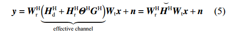
where
The BS can produce the pre-processing matrix
Due to the delay between the channel estimation and data transmission, the pre-processing matrix is set to

with
We propose a new “SVD-ZF” architecture to suppress the ISI resulting from the O-CSI, as depicted in Fig. 1.
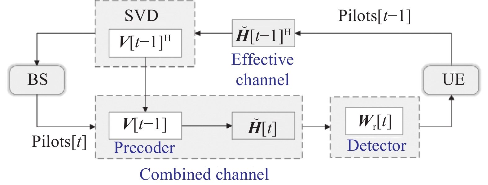
Figure 1. Proposed SVD-ZF scheme over a time-varying channel
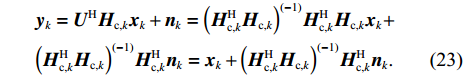
Specifically, given the IRS configuration at a frame, the UE transmits the pilots to the BS at each time slot. Then the BS estimates the I-CSI

Therefore, the decoded signal is given by

The signal-to-interference-plus-noise ratio (SINR) of the mth data stream is given by

2.3 Beamforming strategy and problem formulation
The IRS-related cascaded channel needs to be estimated, every time the IRS is reconfigured. Consequently, the channel estimation would require large training and feedback overhead, if the IRS phase shifts are updated slot by slot.
We propose a TTSBF strategy, which configures the IRS once per frame based on the S-CSI and updates the beamformers frequently every slot according to the O-CSI. As illustrated in Fig. 2, within each frame, the large-scale fading
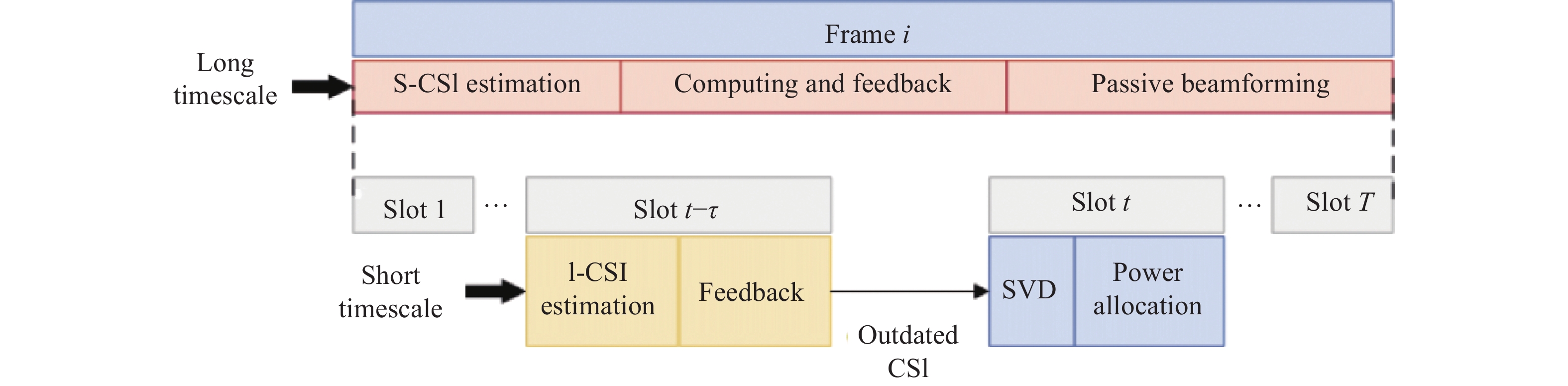
Figure 2. Graphical illustration of TTSBF strategy
Under the SVD-ZF scheme, a short-timescale power allocation method is designed to accommodate the fixed PBF of the IRS as follows:
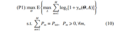

where the constraint in (10) guarantees that the total transmit power of the BS does not exceed its power budget
In this section, we reformulate problem (P1) as a joint design of power allocation at the BS and PBF at the IRS, and design a new modified PSO algorithm to solve it efficiently.
We first rewrite the SINR of the mth data stream at slot t,

Denoting
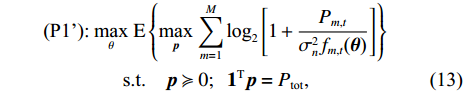

where
Problem (P1 ’) is a stochastic optimization problem, because of the per-slot optimization of the power allocation. At each slot, the power allocation is based on O-CSI, and the fixed phase-shifts of the IRS configured at the long timescale. The IRS PBF optimization needs to predictively maximize the expectation of the sum-rate over random channel samples and potential per-slot power allocations throughout the frame. Although we can transforms Problem (P1 ’) into a deterministic optimization problem, it confronts serious challenges: lack of explicit relation between
The key problem decomposition and the associated schemes are summarized in Fig. 3.
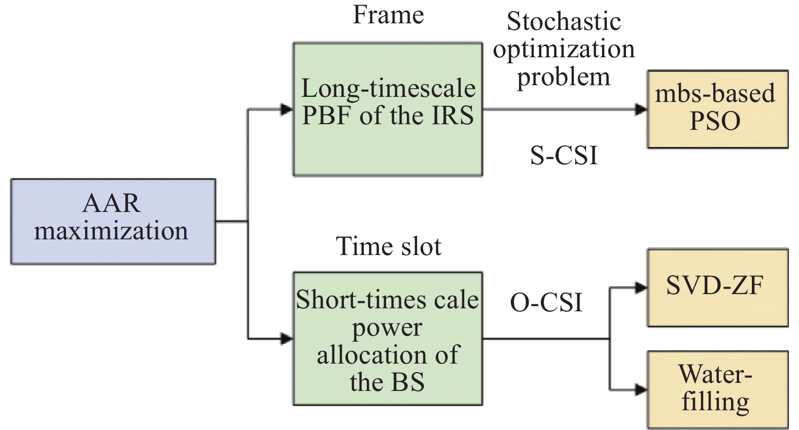
Figure 3. An overview of the proposed twin-timescale resource alloca-tion scheme
3.1 Short-timescale power allocation scheme
Provided that the PBF of the IRS (i.e., the IRS configuration) is optimized at the beginning of the current frame, problem (P1) is written as

Problem (P2) is convex with respect to
where

with
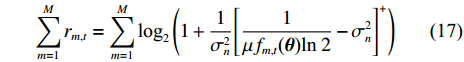
where
3.2 Long-timescale PBF design
The per-frame PBF is a stochastic optimization problem due to the expectation operation in the objective of Problem (P1 ’). To circumvent this impasse, we first rewrite the objective in a deterministic form. Specifically, we take the average rate of
The lth channel sample set in the tth time slot is collected by
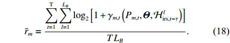
The long-timescale PBF problem is rewritten as

Apart from the nonconvex constant-modulus constraint, the power allocation variables are closely coupled with the reflection phase-shifts of the IRS. As
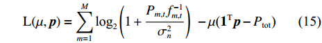
We propose a new PSO framework to solve problem (P3). The PSO, a widely-used meta-heuristic bionic optimization algorithm [12], can find the optimal solution with the benefits of fewer parameters, simple calculation implementation, and fast convergence [13]. In the PSO method, the position of each particle stands for a potential solution. The fitness function of the particle is typically defined to be the optimization objective. We define an IRS refection angle vector

According to (15), for each particle
The global optimal position is selected from the best positions of all particles. Let


where w is the nonnegative inertia weight of a particle;
Each particle requires a notable amount of calculations for the fitness function evaluation per iteration, as the fitness function is evaluated over large number of random channel samples. It can be computationally prohibitive to take all channel samples (which are generally high-dimensional matrices, e.g.,
We develop an mbs-PSO algorithm which is able to substantially reduce the number of channel samples used to evaluate the fitness function while reaping satisfactory performance. Specifically, we introduce a mini-batch recursive sampling surrogate function to replace the fitness function in (17). All
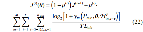
where
From (12), it is seen that the main operations for each particle that contributes to the computational complexity lies on one matrix addition, four matrix multiplications and one matrix inversion using one channel sample. The overall computational complexity of the proposed mbs-PSO algorithm is scaled with a
In practical, the PSO algorithm is deployed at the BS and then informs the instructions to the UE via the IRS controller. As the BS server exhibits the powerful computational capability, a real-time IRS configuration can be enabled. In addition, a moderate number of particles and iterations are generally required to achieve a desirable performance. Moreover, the calculations dominating by the fitness evaluation can be simply parallelized through pipelining in the field programmable gate array (FPGA) [14, 15], which is promising to guarantee strict real-time applications.
Remark 1 In the proposed mbs-PSO algorithm, the fitness function represents the AAR objective. The positions of all particles represent the potential PBF solutions, which are updated by evaluating the fitness value in each iteration. Note that the optimal positions are recorded by comparing with the historical fitness values. This results in a monotonically non-decreasing sequence of AAR values with corresponding PBF solutions updated. On the other hand, the AAR is upper bounded due to the finite transmit powers. Therefore, the convergence can be guaranteed.
Our proposed method for the point-to-point MIMO system can be easily extended to the multi-user MIMO system. This is because the multi-user MIMO channel can be decomposed into parallel single-user MIMO channels by the classical block diagonalization (BD) technique [16]. Therefore, the proposed algorithm can still be valid for each single-user MIMO channel.
To be specific, in the K-user MIMO model, the combined channel matrix is given by
It is seen that this signal model is similar to that under the single-user MIMO scenario. Consequently, the following PBF and power allocation problems can also be solved by the proposed method.
Simulation results are provided to evaluate the performance of our proposed method, including the transmission architecture and optimization algorithm. In the simulations, the path loss model is set according to
Five baselines are used for comparison, which is given as follows: (i) Upper bound: the PSO method is performed by using the AAR object in (P3) as the fitness function where each iteration requires large-scale channel samples. (ii) Sum-path-gain maximization (SPGM)-based scheme [17]: the long-term reflection matrix is obtained via the SPGM-based optimization method. (iii) SVD-based scheme: we adopt the conventional SVD-based MIMO processing architecture, where the transmit powers are optimized by considering the O-CSI as the ideal CSI in each slot. (iv) Random phase: based on the SVD-ZF, we adopt the randomly generated long-term reflection matrix to optimize the transmit powers by using (15). (v) Without IRS: based on the SVD-ZF, we just optimize the transmit powers to optimize the overall sum rate in one frame.
Fig. 4 shows the convergence behaviors of the proposed mbs-PSO algorithm. Note that the original AAR is not set as its fitness objective. From the fitness value results, we see that the mbs-PSO algorithm exhibits the good convergence. More importantly, the sampling surrogate function is effective, as the corresponding AAR is significantly improved during iterations.
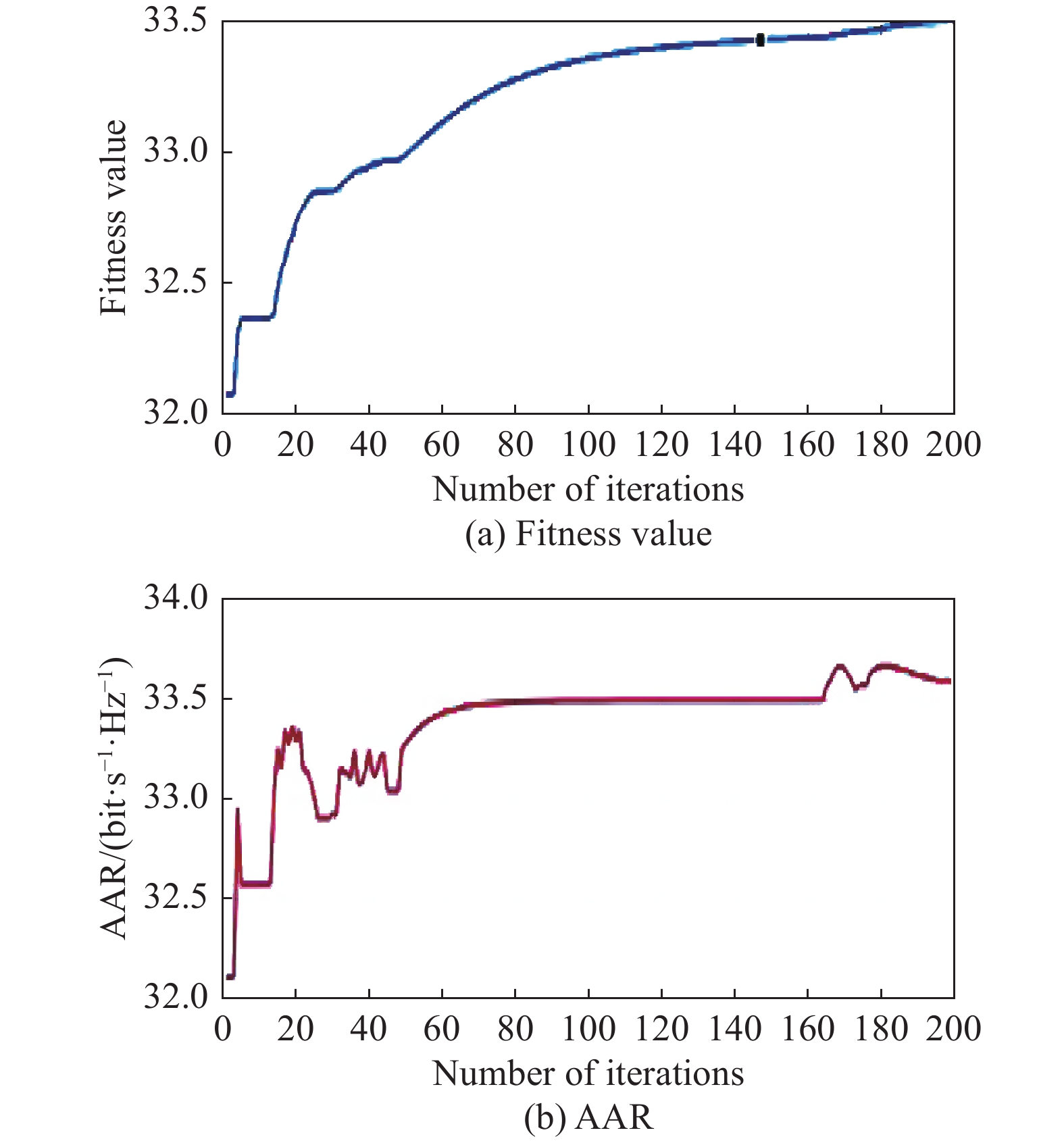
Figure 4. Convergence behaviors of proposed algorithm
Fig. 5 shows the impact of different mini-batch sizes on the convergent AAR. It is observed that all proposed algorithms with different Lmb values can converge within 200 iterations. As can be seen in the top subfigure, the proposed algorithm with small Lmb values exhibits a slight improvement of fitness gap, while the algorithm can gain a sharp improvement with large Lmb values. Comparing the two subfigures, however, we see that the subfigures do not exhibit the same upward trend. In particular, the bottom subfigure does not show a monotonic curve. This is reasonable because of the stochastic nature of the considered mini-batch sampling surrogate function.
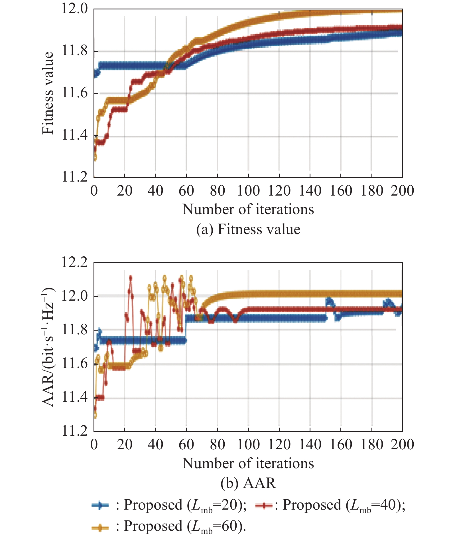
Figure 5. AAR versus mini-batch size
In Fig. 6, we compare different schemes under varying total powers. As
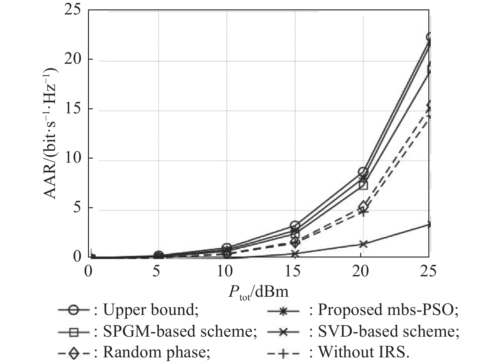
Figure 6. AAR versus total transmit power under different schemes
In Fig. 7, the AAR is plotted against the number of BS antennas, where the number of receive antennas is fixed as Nu = 4. It is seen that the AAR curves for all schemes show an approximately logarithmic shape. Although the number of receive antennas keeps constant, more transmit antennas can still provide a higher spatial diversity gain in the downlink transmission. Hence, the sum rate is improved with the increasing transmit antennas because the downlink SINR is increased. Also, the SPGM-based method performs the worse among all methods, which is consistent with the results in Fig. 6.
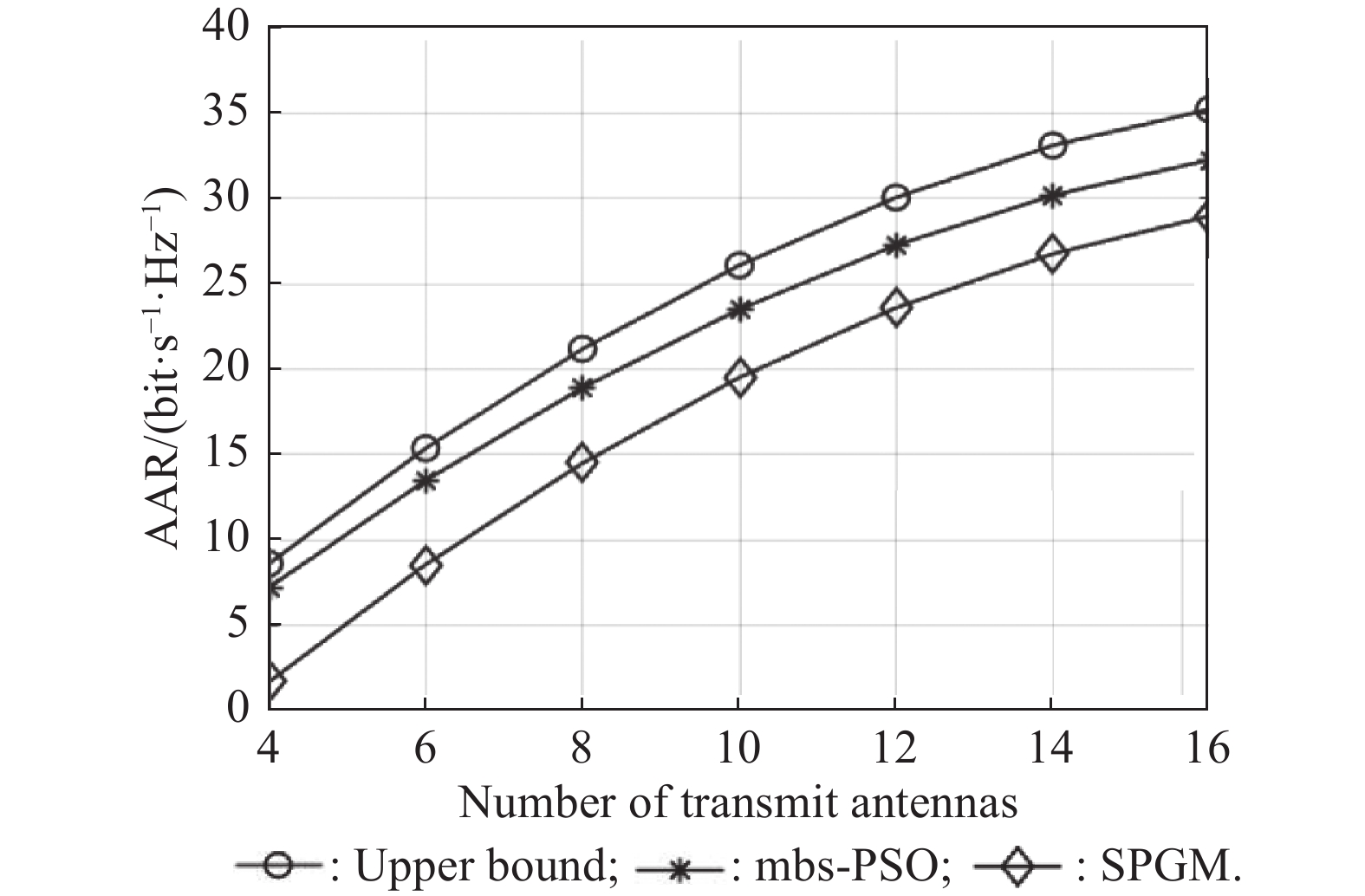
Figure 7. AAR versus the number of BS antennas
Fig. 8 investigates the impact of O-CSI effect on the system AAR. From (4), as the time delay
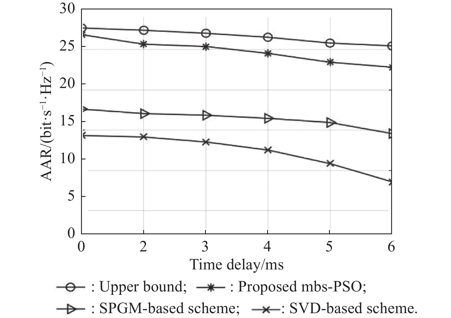
Figure 8. AAR versus time delay
This paper develops an SVD-ZF-based transmission strategy to overcome the O-CSI in the considered IRS-assisted MIMO system. Since frequent IRS reconfigurations would incur large feedback overhead, we propose a TTSBF protocol, where the PBF at the IRS is designed in the long-timescale, while the BS power allocation is performed based on the O-CSI in each short-timescale slot. Particularly, the power allocation is derived with the closed-form water-filling solutions. Then, an mbs-PSO algorithm is proposed to efficiently solve the long-timescale PBF. Finally, we evaluate the proposed transmission strategy and PSO algorithms by comparing multiple baselines.